
The normal distribution is the holy grail of anomaly detection. Normally distributed metrics follow a set of probabilistic rules. Values that follow those rules are recognized as being “normal” or “usual”, while values that break them are seen as being unusual, indicating anomalies.
What is a Normal Distribution ?
Definition
A normal distribution is a very common probability distribution that approximates the behavior of many natural phenomena. A data set is known as “normally distributed” when most of the data aggregates around its mean in a symmetric fashion. Values become less and less likely to occur the farther they are from the mean.
Example of a Normal Distribution
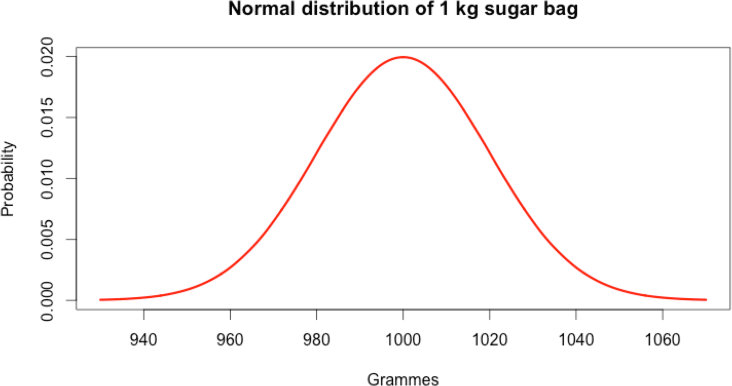
A factory producing 1 kg bags of sugar won’t always make each exactly 1 kg. In reality, the bags are around 1 kg. Most of the time they will be very close to 1 kg, and very rarely far from that figure.
Indeed, the production of 1 kg bags of sugar follows a normal distribution.
Mathematical Rules
When a metric is normally distributed it follows some interesting laws, as in the sugar bag example.
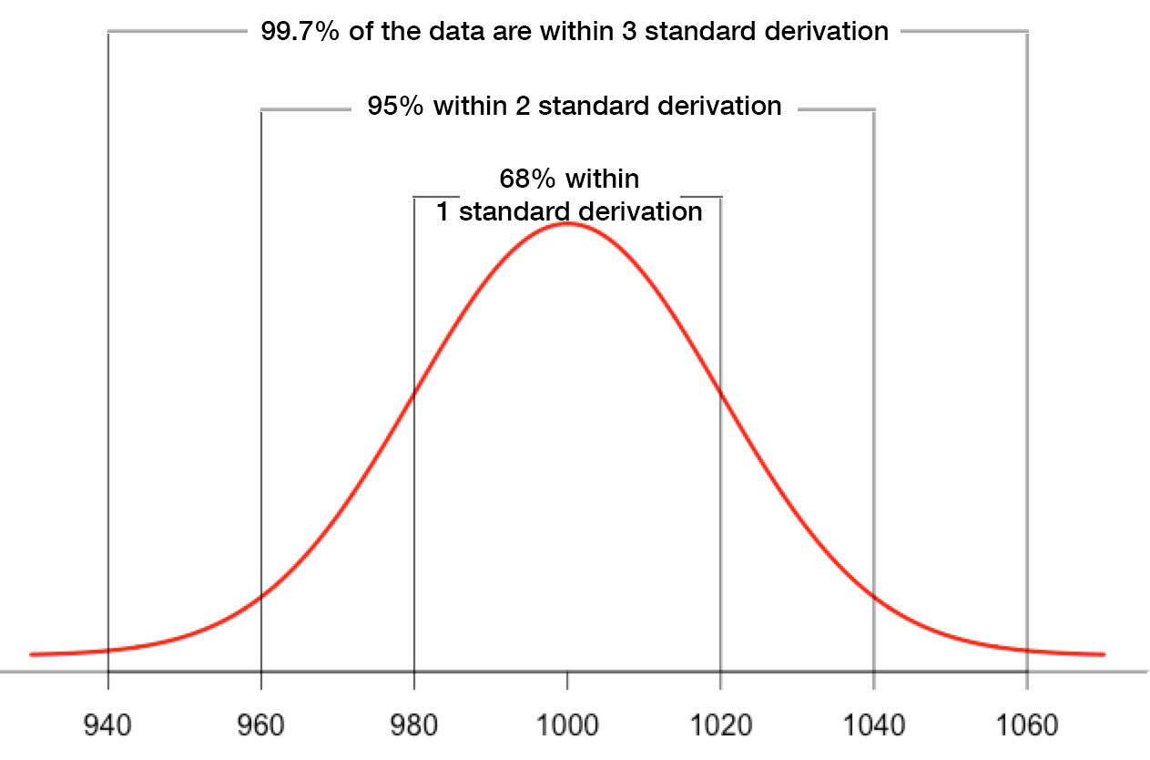
- The mean and the median are the same: both are equal to 1000 in this case. This is because of the perfectly symmetric “bell-shape”.
- The standard deviation, called sigma (σ), defines how far the normal distribution is spread around the mean. In this example σ = 20.
- 68% of all values fall between [mean-σ, mean+σ]; for the sugar bag this is [980, 1020].
- 95% of all values fall between [mean-2*σ, mean+2*σ]; for the sugar bag, [960, 1040].
- 99,7% of all values fall between [mean-3*σ, mean+3*σ]; in the sugar bag example, [940; 1060].
The last 3 rules are also known as the 68–95–99.7 rule or the “three-sigma rule of thumb”.
When the Rules are Broken, It’s an Anomaly
When a system has been proven to be normally distributed, it follows a set of rules as described above. Those rules become the model representing the normal behaviour of the metric. Under normal conditions, values will match the normal distribution and the model will be followed properly. But what happens when the rules get broken? This is when things turn ugly, indicating that something unusual is happening.
In theory, in a normal distribution, no values are impossible. If the weight of the bag of sugar was really normally distributed (it isn’t, this is just an example) we would probably find that 1 out of every billion or so bags of sugar is actually only 860 g. In reality, we approximate this sugar bag example as normally distributed. Almost impossible values are also approximated to be impossible.
Detecting Anomalies – The Theory
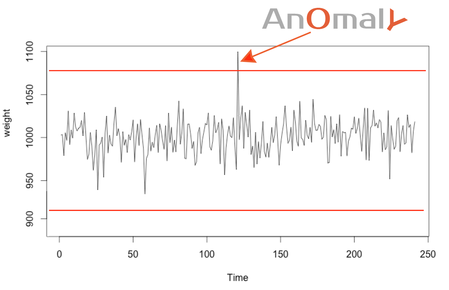
Technique #1: Outlier Values
Almost impossible values can be considered anomalies. When the value deviates too much from the mean, let’s say by ± 4σ, then we can considerate this almost impossible value to be anomalous. (This limit can also be calculated using the percentile.)
For example, sugar bags that weighs less than 920 g or more than 1080 g are considered anomalous. Chances are that these indicate a problem in the production process.
This is a simple way to define maximum and minimum thresholds.
Technique #2: Detecting Rare Distributions
Measured values should respect the 68–95–99.7 rule. If the normal distribution changes, then something unusual has occurred.
As the previous rule states, there is only a 0.3% chance of a value falling outside 3rd sigma range (3σ). Which mean the chance that 4 following values fall consecutively in that range is is 8.1-11% (0.003^4). This occurs so rarely that it almost always represents a problem.
Based on the same rules, there is a 68% chance that a value falls within 1 sigma (σ) of the mean. Having 50 values fall consecutively in the 1st sigma range occurs with a probability of 6.13-10% (0.68^55 ). This too is so rare that we expect this to be anomalous.
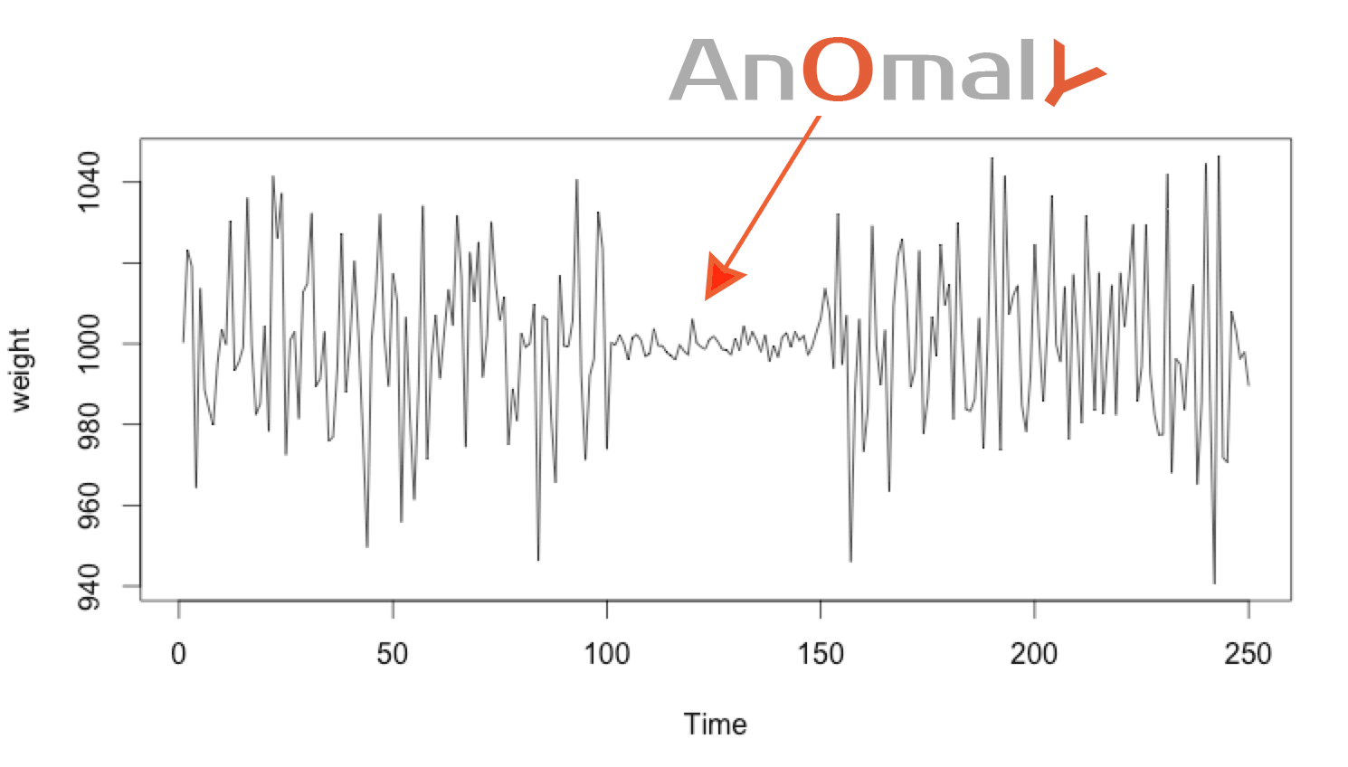
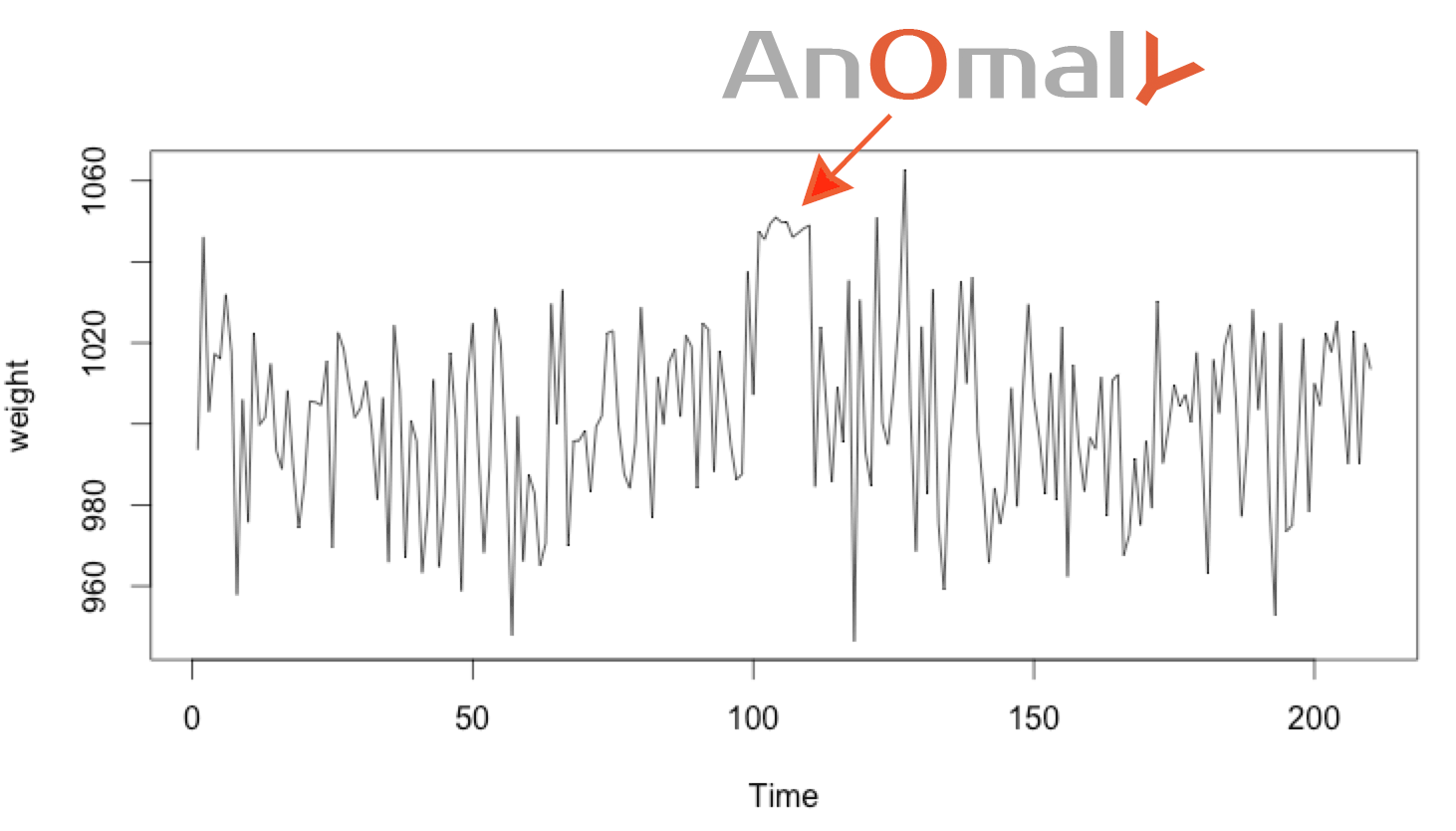
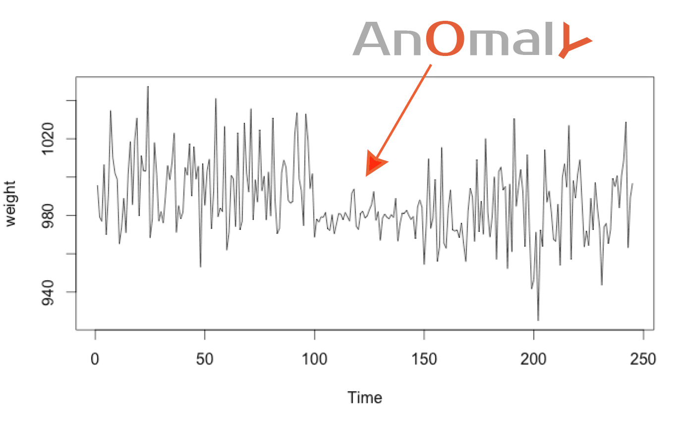
Technique #3: Detecting a Change in the Normal Distribution
Technique #2 can detect unusual distributions quickly, using only a few points. But it can’t detect anomalies that move from one sigma σ to another in an unusual manner.
To detect this kind of anomaly we use a “window” containing the n most recent elements. If the mean and standard derivation of this window change too much from their expected values, we can deduce an anomaly. The bigger the window used, the more stable the anomaly detection, but the more time that is required to detect the anomaly (since it needs to aggregate more value for the detection).
Anomaly Detection – In Practice
In nature, many process are normally distributed. Sadly, in server monitoring, metrics aren’t always so well-behaved. For example, here is the CPU load of my server processing mathematical computations at constant load.
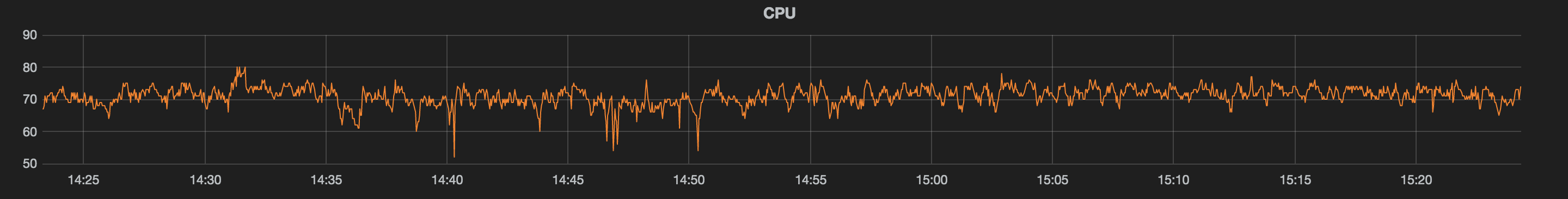
At first glance this CPU graph look to be normally distributed with a mean of around 70, but this hypothesis needs to be confirmed. There are many normality tests to detect if the data is normally distributed. A naive approach is to simply plot the histogram‘s metrics. If it looks bell-shaped, we can approximate the metric as being normally distributed.
Plot of the histogram in R:
1 | cpu |
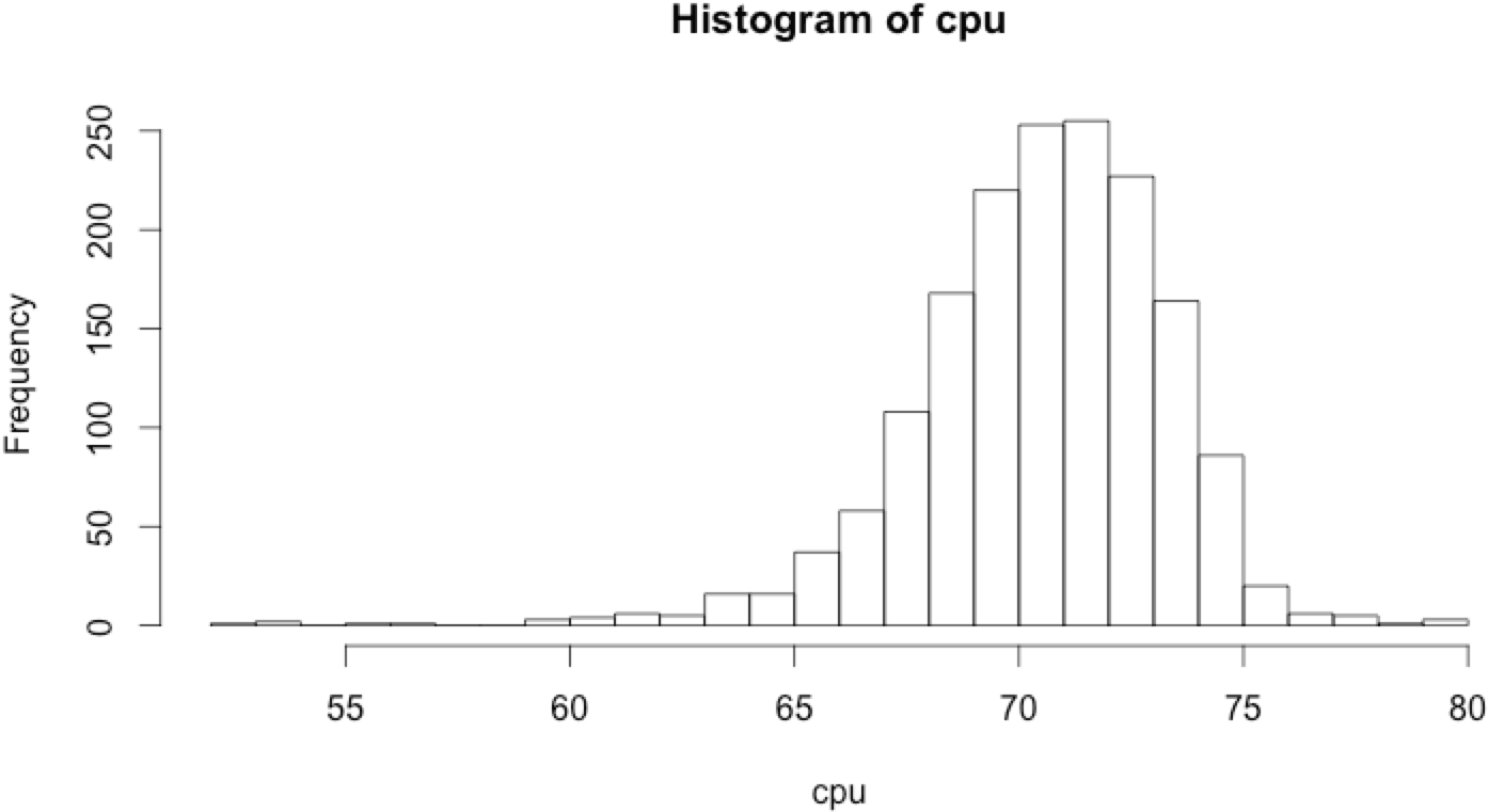
Based on the histogram, the CPU metric is almost normally distributed. So it can be approximated as being normally distributed. As the approximation is relatively crude, the model needs to be more flexible if we don’t want to end up with false alerts all the time.
Applying Technique #1: Outlier Values
To determine almost impossible values we need to calculate the mean and standard deviation of this metric. This is easy using the R language:
1 2 | mean(cpu) # display 70.9982 sd(cpu) # display 2.82513 |
Based on the normal distribution properties, values lower than mean – 4 * standard deviation and higher than mean + 4 * standard deviation should be extremely rare. So the CPU level shouldn’t go under 59.698 nor higher than 82.299. This provides us with some basic thresholds that we can set.
This is represented in the R language by:
1 2 3 | min max ) { print("anomaly !"); } |
Applying Technique #2: Detecting Rare Distributions
Based on the probability distribution it should be very rare when successive values fall within the same sigma. When very rare instances become “almost impossible,” we have an anomaly.
It is (almost) impossible to have:
- 50 consecutive values fall in the 1st sigma
- 7 consecutive values fall in the 2nd sigma
- 4 consecutive values fall in the 3nd sigma
Simple implementation in R:
1 2 3 4 5 6 7 8 9 10 | sigma1max = 50) print("anomaly sigma1"); }else if(sigma2min < point && point < sigma2max){ sigma1count = 8) print("anomaly sigma2"); }else if(sigma3min < point && point < sigma3max){ sigma1count = 4) print("anomaly sigma3"); } } |
On this CPU data set a few false positives occurred, because in reality, this data isn’t exactly normally distributed. To obtain fewer false positives, simply make the rules more flexible.
Applying Technique #3: Detecting a Change in the Normal Distribution
When the standard deviation or the mean change, something unusual is happening. To detect such changes, for each upcoming point “p” we create of window from “p” to “p-100″. Then, we calculate the standard deviation and mean of this window. If it changes too much, an anomaly has been detected.
Here is a simple implementation in R:
1 | usualMean |
detectAnomaly() will not detect any anomaly in the CPU data set:
1 2 | #no output detectAnomaly(cpu, usualMeanMin, usualMeanMax, usualSdMin, usualSdMax); |
detectAnomaly() will detect anomalies when the mean changed from the usual:
1 2 3 | #should detect "mean anomaly" set.seed(1234); cpu_anomalyMean |
detectAnomaly() will detect when the standard deviation changed from the usual:
1 2 3 | #should detect "sd anomaly" set.seed(1234); cpu_anomalySD |
Conclusion
This is just an overview of a few anomaly detection techniques we can use with normally distributed metrics. Sadly, in server monitoring, data isn’t often normally distributed, rather following a seasonal pattern where the model changes every hour, day or week. The number of pageviews on a traditional website, for example, won’t be the same from 2 to 3 am as they are between 7 and 8 pm.
Still, the normal distribution is often used in server monitoring. This is because many anomaly detection methods involve subtracting the model from the real data. The remainder is some noise, due to randomness, which is not normally distributed. The final step is to check this noise distribution to detect anomalies, using the same methods described in this article.
Monitor & detect anomalies with Anomaly.io
SIGN UP sending...
Pingback: Anomaly Detection using K-Means Clustering - Anomaly()