
Monitored metrics very often exhibit regular patterns. When the values are correlated with the time of the day, it’s easier to spot anomalies, but it’s harder when they do not. In some cases, it is possible to use machine learning to differentiate the usual patterns from the unusual ones.
Regular Patterns
Many metrics follow regular patterns correlated to time. Websites, for example, commonly experience high activity during the day and low activity at night. This correlation with time makes it easy to spot anomalies, but it’s more difficult when that correlation is not present.
1. With Time Correlation
When the metric is correlated to time, the key point is to find its seasonality. When today’s pattern is the same as yesterday, the seasonality is daily. It is also common to find seasonality of one week because Saturday’s patterns often don’t follow Friday’s, but rather those of the Saturday of the previous week. Because many metrics are correlated to human activity, seasonality is often weekly. But it could also be measured in seconds, minutes, hours, month or an arbitrary period.
Subtracting the usual pattern (seasonality) from the overall signal should create a new “difference metric”. Due to randomness, the resulting signal should be pure noise with a mean of zero. Under such conditions, we can apply the normal distribution to detect anomalies. Any values that are too high or too low can be treated as anomalous.
2.Without Time Correlation
A heartbeat has many recurring patterns. The heart beats on average every 0.8s, but this is an average period, not a fixed period of time. Moreover, the period and the value of the signal might change a lot due to physical activity, stress or other effects. So it isn’t possible to just use a period of 0.8 seconds.
So what can we do? Machine learning to the rescue!
Machine Learning Detection
We can group similar patterns into categories using machine learning. Then, we subtract each new beat with its closest category. If the original beat and the category beat are very similar, the result should be pure noise with a mean of zero. As above, it’s now possible to apply the normal distribution to detect anomalies. For an anomalous beat, even the closest category will still be very different. The anomaly will be easy to detect as it will create a peak in the “difference metric”.
This requires 4 steps:
1. Sliding Window
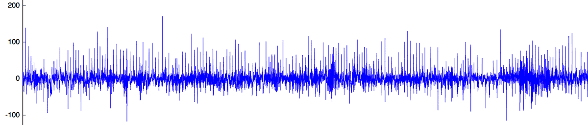
The first step is to “cut” the normal heartbeat signal into smaller chunks. To get better results later, we are going to use a sliding window with an overlap of 50%. For each window, we will apply a Hamming function to clean the signal.
In the following heartbeat implementation, we choose a sliding windows of 60 values represented with a red rectangle. So, we will move the window by 30 values. For each window, we multiply the heartbeat signal (in green) by the hamming function (in red). The end result (in green) is saved to create categories in the next step.
2. Clustering
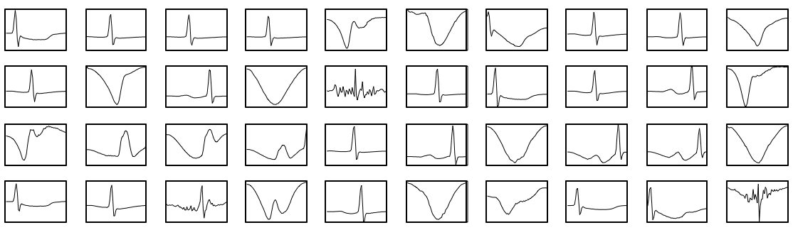
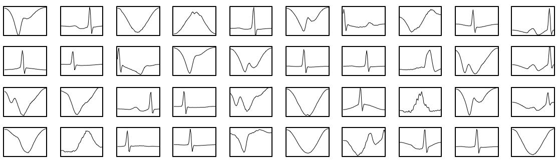
The next step is to group together similar patterns produced by the sliding window. We will use one machine learning technique known as k-means clustering using Matlab/Octave or Mahout. This will cluster our signal into a catalogue of 1000 categories. In the following schema, some categories are plotted.
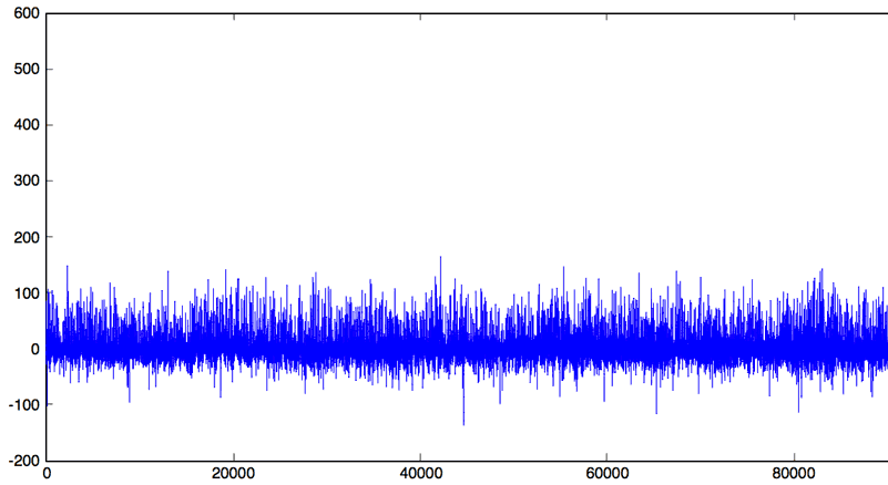
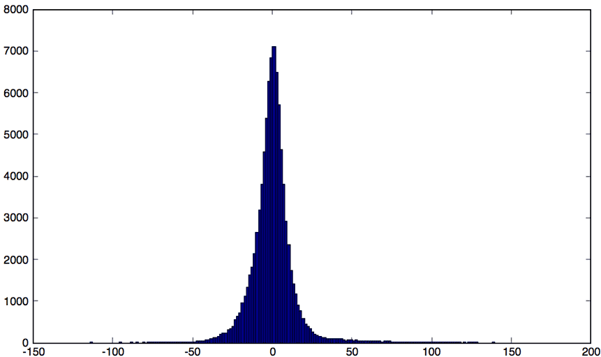
3. Noise Transform
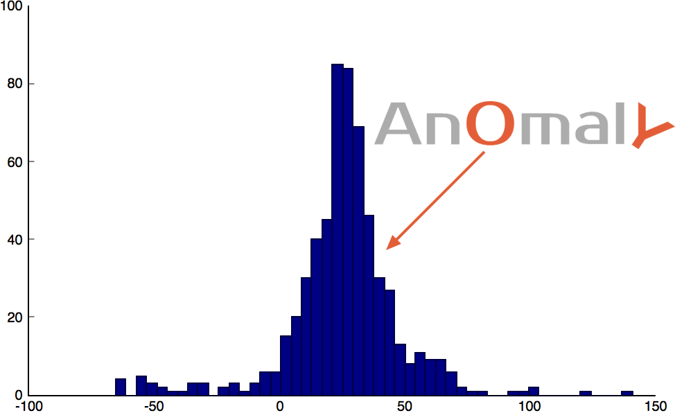
For each sliding window, we select the closest category from our catalogue of patterns created previously. Subtracting the sliding window from its category should produce a simple noisy signal. If the signal is repeating and enough clusters were chosen, the whole signal can be turned into a normally distributed noisy signal with a mean of zero . Because this noisy signal is normally distributed we can apply the normal distribution to detect anomalies. We can plot its histogram, or use the 99.999% percentile, while highlighting the threshold limit to apply on the noisy signal.
4. Detect Anomalies
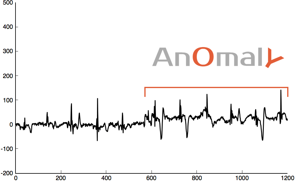
For each new sliding window, we repeat the above process to turn it into a noise signal. Previously we defined minimum and maximum thresholds. The noisy sliding window should be within those limits; if not, this is an anomaly! But that’s not all. We also defined the noise signal as being normally distributed with a mean of zero. If it suddenly changes into another distribution, something unusual or anomalous is appending.
 Min / Max anomaly
 distribution anomaly
 distribution anomaly
Implementation
1. Requirement
First, you need to download and install Octave (recommended) or Matlab. A few packages are will be used in this tutorial. Open an Octave or Matlab shell, install and import these packages:
1 2 3 4 5 6 7 8 9 | % Install package pkg install -forge io pkg install -forge statistics pkg install -forge control pkg install -forge signal % Import package pkg load signal pkg load statistics |
2. Sliding Window
You could use the WFDB Toolbox from physionet.org to download a heartbeat signal and convert it into Octave/Matlab format. But as it’s easier to simply download the converted file “16773m.mat”
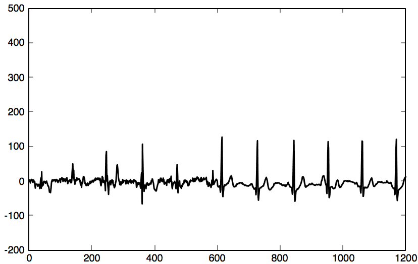
Load the signal in Octave/Matlab , convert into sliding windows, and apply the Hamming function:
1 2 3 4 5 6 7 8 9 10 11 12 13 14 15 16 17 18 19 | % change with your own path cd /path/to/16773m.mat % load & plot some heartbeat signal = load("16773m.mat").val(1,:); plot(signal(1:1000)) % convert to sliding windows % http://www.mathworks.com/help/signal/ref/buffer.html windows = buffer(signal, 60, 30); % apply hamming function % http://www.mathworks.com/help/dsp/ref/windowfunction.html mutate = windows.*hamming(60); points = mutate.'; cleanPoints = points(2:end-1, :); % save for Mahout dlmwrite('heatbeat.txt',cleanPoints,'delimiter',' ','precision','%.4f'); |
All sliding windows are saved in memory into the “cleanPoints” variable and also the “heatbeat.txt” text file. The variable will be used for clustering into Octave/Matlab; the text file will be used for clustering using Mahout.
3. Clustering
Let’s now find common patterns from the signal. We will use the k-means clustering technique, which is part of the machine learning field. It works by grouping together points based on their nearest mean.
.

.
3.1. Clustering with Octave or Matlab
When data can fit into RAM, Octave or Matlab is a good choice. When clustering a small quantity of data, such as this heartbeat signal, you should use Octave or Matlab.
Octave and Matlab come with a k-means implementation in the statistics package. As it’s quite slow we will use a faster implementation call Fast K-means. Download fkmeans.m and save the file into the directory of your Octave / Matlab workspace. Use the “pwd” command to find your workspace path.
If you save fkmeans.m in your current workspace, you should be able to create 1000 clusters:
1 | [~, clusters, ~] = fkmeans(cleanPoints, 1000); |
It should take around 30 minutes, so let’s save the file, just in case.
1 | save "1000_clusters_fkmeans.mat" clusters -ascii; |
If you have any trouble creating this file, you can download 1000_clusters_fkmeans.mat and simply load it within Octave or Matlab:
1 | clusters = load("1000_clusters_fkmeans.mat"); |
3.2. Clustering with Mahout
When the data you went to cluster is huge and won’t fit into memory, you should choose a tool designed for this use case, such as Mahout.
First, download and install Mahout. Previously we created a file call “heatbeat.txt” containing all the sliding windows. You have to copy this file into a directory call “testdata”. Then, run the Mahout clustering from your shell:
1 2 3 | mkdir testdata cp /path/to/heatbeat.txt testdata/ mahout org.apache.mahout.clustering.syntheticcontrol.kmeans.Job --input testdata --output out_1000 --numClusters 1000 --t1 200 --t2 100 --maxIter 50 |
A few hours later, the clustering result will be written into the “out_1000″ directory. Now export the Mahout result into Octave or Matlab. Let’s use cluster2csv.jar to convert this Mahout file into a CSV file.
1 | java -jar cluster2csv.jar out_1000/clusters-50-final/part-r-00000 > 1000_clusters_mahout.csv |
Finaly, let’s import 1000_clusters_mahout.csv into Octave or Matlab:
1 | clusters = load("1000_clusters_fkmeans.mat"); |
4. Noise Transform
To transform the original signal into a noise signal, we need a few steps. First, we need a function that can find the closest cluster for a given signal window:
1 2 3 4 5 6 7 8 9 10 | function clusterIndices = nearKmean(clusters, data) numObservarations = size(data)(1); K = size(clusters)(1); D = zeros(numObservarations, K); for k=1:K %d = sum((x-y).^2).^0.5 D(:,k) = sum( ((data - repmat(clusters(k,:),numObservarations,1)).^2), 2); end [minDists, clusterIndices] = min(D, [], 2); end |
We need to subtract the window from the closest cluster:
1 2 3 4 5 6 7 8 9 | function diffWindows = diffKmean(clusterIndices, clusters, data) diffWindows = []; for i = 1:length(clusterIndices) entry = data(i,:); cluster = clusters(clusterIndices(i),:); diff = cluster-entry; diffWindows = [diffWindows; diff]; end end |
And finally, a function to reconstruct the “difference signal”, also call the “error signal”:
1 2 3 4 5 6 | function reconstruct = asSignal(diffWindows) rDiffWindows = diffWindows.'; p1 = rDiffWindows(1:size(rDiffWindows,1)/2,2:end); p2 = rDiffWindows((size(rDiffWindows,1)/2)+1:size(rDiffWindows,1),1:end-1); reconstruct = reshape(p1.+p2, [], 1)(:)'; end |
With a sample, let’s apply the above function to draw the error signal:
1 2 3 4 5 6 | samples = cleanPoints(20200:20800, :); clusterIndices = nearKmean(clusters, samples); diffWindows = diffKmean(clusterIndices, clusters, samples); reconstructDelta = asSignal(diffWindows); plot(reconstructDelta) ylim ([-200 600]) |
5. Detect Anomaly
Let’s simulate the beginning of a heart attack and detect the anomaly.
1 2 3 4 5 6 7 8 9 10 | attack = cleanPoints(10002, :); attack(35:43) = [100,350,325,250,410,380,300,200,100]; clusterId = nearKmean(clusters, attack); cluster = clusters(clusterId,:); plot(attack, "linewidth",1.5, 'Color', [0.1484375,0.7578125,0.71484375]); ylim([-200 500]); hold on; plot(cluster, "linewidth",1.5, 'Color', [0.875486381,0.37109375,0.24609375]); hold off; |
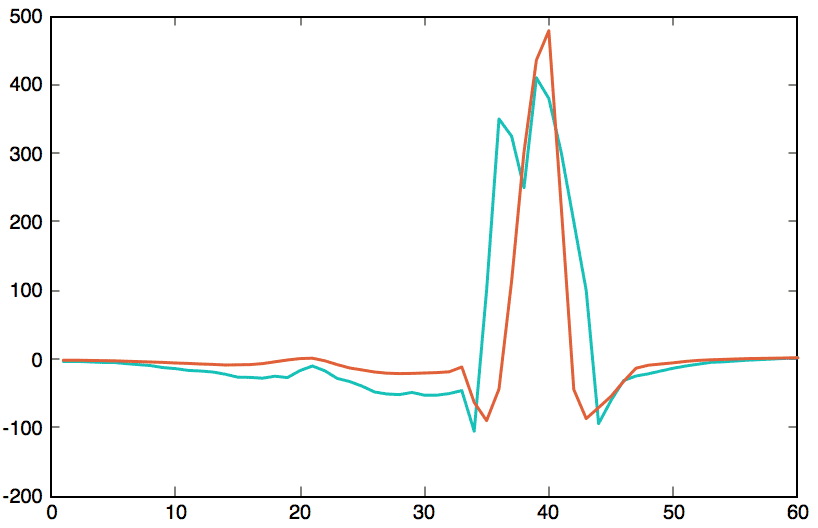
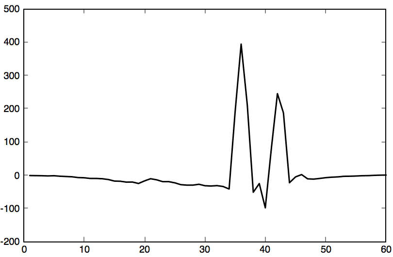
Clearly, there is a huge difference between the heart attack and its closest pattern. This plot highlights the anomaly.
1 2 3 | diff = attack-cluster; plot(diff, "linewidth",1.5, 'Color', "black"); ylim([-200 500]); |
Previously we established more rules than a simple minimum and maximum. The noisy “error signal” should follow a mean of zero with a specific normal distribution. Let’s simulate this kind of dysfunction.
1 2 3 4 5 6 7 8 9 | p1 = cleanPoints(10001:10020, :); p2 = cleanPoints(10020:10040, :); p2 = p2.-(p2*1.2)+15; samples = [p1; p2]; clusterIndices = nearKmean(clusters, samples); diffWindows = diffKmean(clusterIndices, clusters, samples); reconstructDelta = asSignal(diffWindows); plot(reconstructDelta, "linewidth",1.5, 'Color', "black"); ylim([-200 500]); |
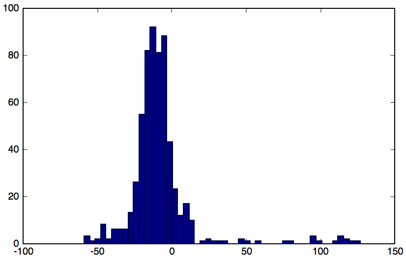
It doesn’t look normally distributed anymore: for sure, it’s not the same distribution as it usually is. It’s an anomaly.
1 2 3 4 5 | clusterIndices = nearKmean(clusters, p2); diffWindows = diffKmean(clusterIndices, clusters, p2); reconstructDelta = asSignal(diffWindows); plot(reconstructDelta, "linewidth",1.5, 'Color', "black"); hist(reconstructDelta, 50); |
Conclusion
This technique is useful only under certain conditions. You should apply this technique if the signal doesn’t repeat itself within a fixed period of time. If it does, such as daily or weekly, it is preferable to simply model the seasonality to detect anomalies.
We have only scratched the surface here when studying the error signal as being normally distributed. In reality there are more ways of detecting anomalies in a normally distributed signal.
Monitor & detect anomalies with Anomaly.io
SIGN UP sending...