To detect the correlation of time series we often use auto-correlation, cross-correlation or normalized cross-correlation. Let’s study these techniques to understand them better.
Definition:
- Cross-correlation is the comparison of two different time series to detect if there is a correlation between metrics with the same maximum and minimum values. For example: “Are two audio signals in phase?”
- Normalized cross-correlation is also the comparison of two time series, but using a different scoring result. Instead of simple cross-correlation, it can compare metrics with different value ranges. For example: “Is there a correlation between the number of customers in the shop and the number of sales per day?”
- Auto-correlation is the comparison of a time series with itself at a different time. It aims, for example, to detect repeating patterns or seasonality. For example: “Is there weekly seasonality on a server website?” “Does the current week’s data highly correlate with that of the previous week?”
- Normalized auto-correlation is the same as normalized cross-correlation, but for auto-correlation, thus comparing one metric with itself at a different time.
- Time Shift can be applied to all of the above algorithms. The idea is to compare a metric to another one with various “shifts in time”. Applying a time shift to the normalized cross-correlation function will result in a “normalized cross-correlation with a time shift of X”. This can be used to answer questions such as: “When many customers come in my shop, do my sales increase 20 minutes later?”
Cross-Correlation
To detect a level of correlation between two signals we use cross-correlation. It is calculated simply by multiplying and summing two-time series together.
In the following example, graphs A and B are cross-correlated but graph C is not correlated to either.
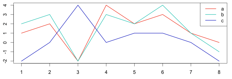
1 2 3 4 5 6 7 8 9 10 | # plot the graph in R a = c(1,2,-2,4,2,3,1,0) b = c(2,3,-2,3,2,4,1,-1) c = c(-2,0,4,0,1,1,0,-2) plot(ts(a), col="#f44e2e", lwd=2) lines(b, col="#27ccc0", lwd=2) lines(c, col="#273ecc", lwd=2) legend("topright", c("a","b","c"), col=c("#f44e2e","#27ccc0","#273ecc"), lty=c(1), lwd = 2) |
Using the cross-correlation formula above we can calculate the level of correlation between series.
$$corr(x, y) = \sum_{n=0}^{n-1} x[n]*y[n]$$
$$\begin{align}
corr(a, b) & = 1*2+2*3+-2*-2+4*3+2*2+3*4+1*1+0*-1 \\
& = 41
\end{align}$$
$$\begin{align}
corr(a, c) & =1*-2+2*0+-2*4+4*0+2*1+3*1+1*0+0*-2 \\
& =-5
\end{align}$$
Graphs A and B correlate, with a high value of 41.
Graphs A and C don’t correlate, having a low value of -5.
1 2 3 | # compute using the R language corr_ab = sum(a*b) # equal 41 corr_ac = sum(a*c) # equal -5 |
Normalized Cross-Correlation
There are three problems with cross-correlation:
- It is difficult to understand the scoring value.
- Both metrics must have the same amplitude. If Graph B has the same shape as Graph A but values two times smaller, the correlation will not be detected.
corr(a, a/2) = 19.5 - Due to the formula, a zero value will not be taken into account, since 0*0=0 and 0*200=0.
To solve these problems we use normalized cross-correlation:
$$norm\_corr(x,y)=\dfrac{\sum_{n=0}^{n-1} x[n]*y[n]}{\sqrt{\sum_{n=0}^{n-1} x[n]^2 * \sum_{n=0}^{n-1} y[n]^2}}$$
Using this formula let’s compute the normalized cross-correlation of AB and AC.
$$\begin{align}
norm\_corr(a,b) &= \dfrac{1*2+2*3+-2*-2+4*3+2*2+3*4+1*1+0*-1}{\sqrt{(1+4+4+16+4+9+1+0)*(4+9+4+9+4+16+1+1)}} \\
& = \dfrac{41}{\sqrt{(39)*(48)}} \\
& = 0.947
\end{align}$$
$$\begin{align}
norm\_corr(a,c) & =\dfrac{1*-2+2*0+-2*4+4*0+2*1+3*1+1*0+0*-2}{\sqrt{(1+4+4+16+4+9+1+0)*(4+0+16+0+1+1+0+4)}} \\
& =\dfrac{-5}{\sqrt{(39)*(26)}} \\
& =-0.157
\end{align}$$
Graphs A and B correlate, with a high value of 0.947.
Graphs A and C don’t correlate, showing a low value of -0.157.
- Normalized cross-correlation scoring is easy to understand:
– The higher the value, the higher the correlation is.
– The maximum value is 1 when two signals are exactly the same:
norm_corr(a,a)=1
– The minimum value is -1 when two signals are exactly opposite:
norm_corr(a, -a) = -1 - Normalized cross-correlation can detect the correlation of two signals with different amplitudes: norma_corr(a, a/2) = 1.
Notice we have perfect correlation between signal A and the same signal with half the amplitude!
1 2 3 | # compute using the R language norm_corr_ab = sum(a*b) / sqrt(sum(a^2)*sum(b^2)) #equal 0.947 norm_corr_ac = sum(a*c) / sqrt(sum(a^2)*sum(c^2)) #equal -0.157 |
Auto-Correlation
Auto-correlation is very useful in many applications; a common one is detecting repeatable patterns due to seasonality.
The following graph clearly shows repeating patterns every 8 data points. Indeed, looking at the R code, it’s a repeatable sequence of the numbers 1 through 8 with some random noise in the mix.

1 2 3 4 | # compute using the R language set.seed(5) ar = rep(c(1,2,3,4,5,6,7,8), 8) + rnorm(8*8, sd = 0.7) plot(ts(ar), col="#f44e2e", lwd=2) |
Let’s compute the auto-correlation between the signal and itself at a time shift of 4 and time shift of 8. The following graphs clearly show a high auto-correlation at time shift 8, but not at time shift 4.
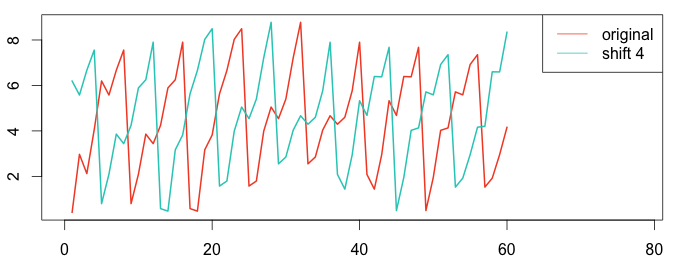
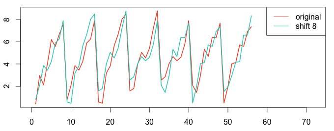
1 2 3 4 5 6 7 8 9 10 11 12 | # plot using the R language ar4 = ar[1:(length(ar)-4)] ar4_shift = ar[5:length(ar)] plot(ts(ar4), col="#f44e2e", lwd=2, xlim=c(0,78)) lines(ar4_shift, col="#27ccc0", lwd=2) legend("topright", c("original","shift 4"), col = c("#f44e2e","#27ccc0"), lty=c(1,1)) ar8 = ar[1:(length(ar)-8)] ar8_shift = ar[9:length(ar)] plot(ts(ar8), col="#f44e2e", lwd=2, xlim=c(0,72)) lines(ar8_shift, col="#27ccc0", lwd=2) legend("topright", c("original","shift 8"), col = c("#f44e2e","#27ccc0"), lty=c(1,1)) |
To compute, we can use the same formula as cross-correlation (see above).
1 2 3 | # compute using the R language corr_arar4 = sum(ar4*ar4_shift) #equals 1130.705 corr_arar8 = sum(ar8*ar8_shift) #equals 1456.428 |
For a time shift of 8 the auto-correlation is higher than a time shift of 4. We have detected seasonality with a period of 8.
Normalized Auto-Correlation
We discussed earlier the advantages of normalized cross-correlation. In the same way, we can compute the normalized auto-correlation with time shifts of 4 and 8:
1 2 3 | # compute using the R language norm_auto_arar4 = sum(ar4*ar4_shift) / sqrt(sum(ar4^2)*sum(ar4_shift^2)) #equal 0.726 norm_auto_arar8 = sum(ar8*ar8_shift) / sqrt(sum(ar8^2)*sum(ar8_shift^2)) #equal 0.981 |
Normalized cross-correlation makes it very obvious that the signal repeats in a similar manner every 8 data points.
Correlation with Time Shift
All correlation techniques can be modified by applying a time shift. For example, it is very common to perform a normalized cross-correlation with time shift to detect if a signal “lags” or “leads” another.
To process a time shift, we correlate the original signal with another one moved by x elements to the right or left. Just as we did for auto-correlation.
To detect if two metrics are correlated with a time shift we need to compute all the possible time shifts. Fortunately, the R language can compute all the correlations with time shift very quickly.
Normalized Cross-Correlation with Time Shift
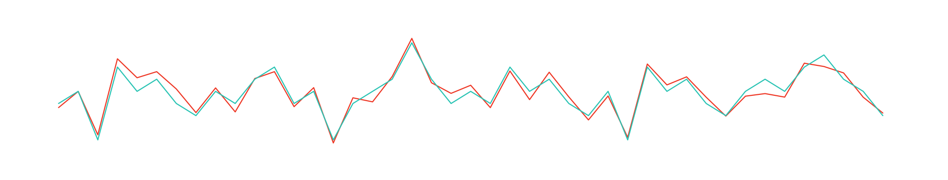
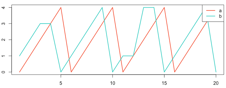
1 2 3 4 5 6 7 8 9 10 11 12 13 14 15 | # using R language library(stats) # Normalized Cross-Correlation for lags from -4 to 4 a = c(0,1,2,3,4,0,1,2,3,4,0,1,2,3,4,0,1,2,3,4) b = c(1,2,3,3,0,1,2,3,4,0,1,1,4,4,0,1,2,3,4,0) #show graph plot(ts(a), col="#f44e2e", lwd=2) lines(b, col="#27ccc0", lwd=2) legend("topright", c("a","b"), col=c("#f44e2e","#27ccc0"), lty=c(1), lwd = 2) r = ccf(a,b, lag.max = 4) r #show correlation values |
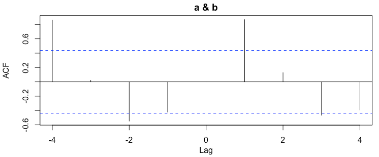
| -4 | -3 | -2 | -1 | 0 | 1 | 2 | 3 | 4 |
| 0.862 | 0.021 | -0.547 | -0.423 | 0.000 | 0.867 | 0.127 | -0.466 | -0.393 |
As we expected from the graph above, the metrics highly correlate with a time shift of 1.
Normalized Auto-Correlation with Time Shift
1 2 3 4 5 6 7 8 9 10 11 12 | # using R language library(stats) # Normalized Auto-Correlation for lags from -10 to 10 set.seed(5) ar = rep(c(1,2,3,4,5,6,7,8), 8) + rnorm(8*8, sd = 0.7) #display plot(ts(ar), col="#f44e2e", lwd=2) r = acf(ar, lag.max = 10) r # show correlation values |
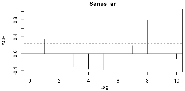
| 0 | 1 | 2 | 3 | 4 | 5 | 6 | 7 | 8 | 9 | 10 |
| 1.000 | 0.335 | -0.122 | -0.304 | -0.369 | -0.374 | -0.226 | 0.187 | 0.789 | 0.306 | -0.120 |
The output above repeats every 8 datapoints. As expected, the auto-correlation detects a high correlation when the series is compared to itself at a time shift of 8.
Conclusion
Here at anomaly.io, we commonly use both cross-correlation and auto-correlation, which are building blocks to detecting unusual patterns in your data. As auto-correlation can detect the seasonality of a metric, we can apply a range of anomaly detection algorithms such as seasonal decomposition of time series or seasonally adjusting a time series. When a cross-correlation is found, we can detect anomalies when the correlation is broken between the series.
Be sure to also read “Detecting Correlation Among Time Series“.
Monitor & detect anomalies with Anomaly.io
SIGN UP sending...