Time series decomposition works by splitting a time series into three components: seasonality, trends and random fluctiation. To show how this works, we will study the decompose( ) and STL( ) functions in the R language.
Understanding Decomposition
Decompose One Time Series into Multiple Series
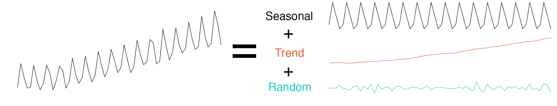
Time series decomposition is a mathematical procedure which transforms a time series into multiple different time series. The original time series is often split into 3 component series:
- Seasonal: Patterns that repeat with a fixed period of time. For example, a website might receive more visits during weekends; this would produce data with a seasonality of 7 days.
- Trend: The underlying trend of the metrics. A website increasing in popularity should show a general trend that goes up.
- Random: Also call “noise”, “irregular” or “remainder,” this is the residuals of the original time series after the seasonal and trend series are removed.
Additive or Multiplicative Decomposition?
To achieve successful decomposition, it is important to choose between the additive and multiplicative models, which requires analyzing the series. For example, does the magnitude of the seasonality increase when the time series increases?
 Australian beer production – The seasonal variation looks constant; it doesn’t change when the time series value increases. We should use the additive model.
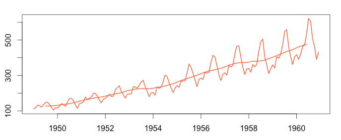
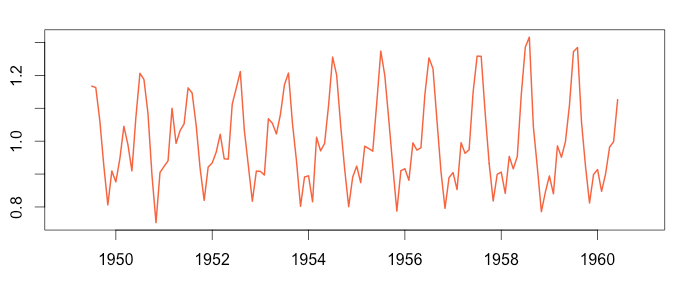
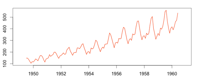
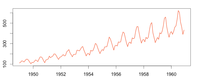 Airline Passenger Numbers – As the time series increases in magnitude, the seasonal variation increases as well. Here we should use the multiplicative model.
Additive:
Time series = Seasonal + Trend + Random
Multiplicative:
Time series = Trend * Seasonal *Random
The decomposition formula varies a little based on the model.
Step-by-Step: Time Series Decomposition
We’ll study the decompose( ) function in R. As a decomposition function, it takes a time series as a parameter and decomposes it into seasonal, trend and random time series. We’ll reproduce step-by-step the decompose( ) function in R to understand how it works. Since there are variations between the two models, we’ll use two examples: Australian beer production (additive) and airline passenger numbers (multiplicative).
Step 1: Import the Data
Additive
As mentioned previously, a good example of additive time series is beer production. As the metric values increase, the seasonality stays relatively constant.
Multiplicative
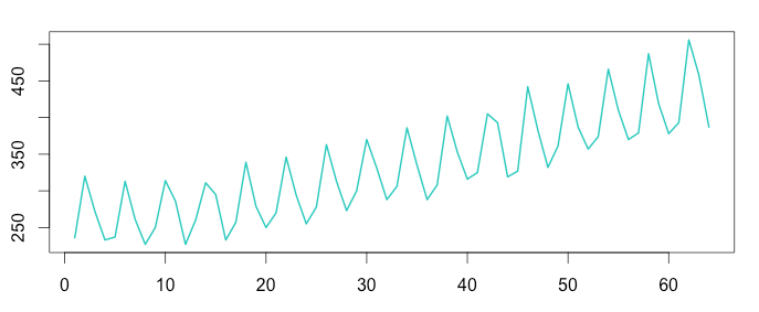
Monthly airline passenger figures are a good example of a multiplicative time series. The more passengers there are, the more seasonality is observed.
1 2 3 4 5 | install.packages("fpp") library(fpp) data(ausbeer) timeserie_beer = tail(head(ausbeer, 17*4+2),17*4-4) plot(as.ts(timeserie_beer)) |
1 2 3 4 5 | install.packages("Ecdat") library(Ecdat) data(AirPassengers) timeserie_air = AirPassengers plot(as.ts(timeserie_air)) |
Step 2: Detect the Trend
To detect the underlying trend, we smoothe the time series using the “centred moving average“. To perform the decomposition, it is vital to use a moving window of the exact size of the seasonality. Therefore, to decompose a time series we need to know the seasonality period: weekly, monthly, etc… If you don’t know this figure, you can detect the seasonality using a Fourier transform.
Additive
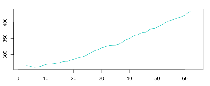
Australian beer production clearly follows annual seasonality. As it is recorded quarterly, there are 4 data points recorded per year, and we use a moving average window of 4.
Multiplicative
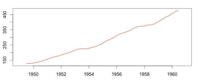
The process here is the same as for the additive model. Airline passenger number seasonality also looks annual. However, it is recorded monthly, so we choose a moving average window of 12.
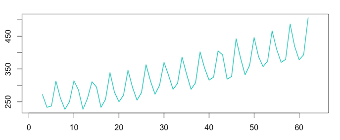
1 2 3 4 5 6 | install.packages("forecast") library(forecast) trend_beer = ma(timeserie_beer, order = 4, centre = T) plot(as.ts(timeserie_beer)) lines(trend_beer) plot(as.ts(trend_beer)) |
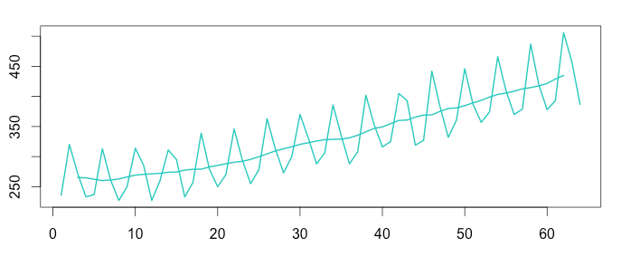
1 2 3 4 5 6 | install.packages("forecast") library(forecast) trend_air = ma(timeserie_air, order = 12, centre = T) plot(as.ts(timeserie_air)) lines(trend_air) plot(as.ts(trend_air)) |
Step 3: Detrend the Time Series
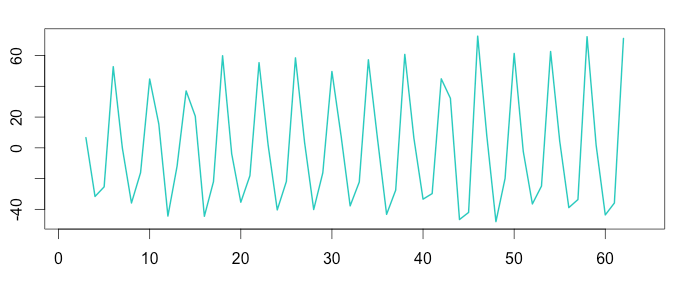
Removing the previously calculated trend from the time series will result into a new time series that clearly exposes seasonality.
Additive
Multiplicative
1 2 | detrend_beer = timeserie_beer - trend_beer plot(as.ts(detrend_beer)) |
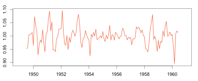
1 2 | detrend_air = timeserie_air / trend_air plot(as.ts(detrend_air)) |
Step 4: Average the Seasonality
From the detrended time series, it’s easy to compute the average seasonality. We add the seasonality together and divide by the seasonality period. Technically speaking, to average together the time series we feed the time series into a matrix. Then, we transform the matrix so each column contains elements of the same period (same day, same month, same quarter, etc…). Finally, we compute the mean of each column. Here is how to do it in R:
Additive
Quarterly seasonality: we use a matrix of 4 rows. The average seasonality is repeated 16 times to create the graphic to be compared later (see below)
Multiplicative
Monthly seasonality: we use a matrix of 12 rows.
The average seasonality is repeated 12 times to create the graphic we will compare later (see below)
1 2 3 | m_beer = t(matrix(data = detrend_beer, nrow = 4)) seasonal_beer = colMeans(m_beer, na.rm = T) plot(as.ts(rep(seasonal_beer,16))) |
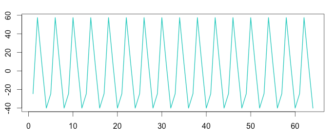
1 2 3 | m_air = t(matrix(data = detrend_air, nrow = 12)) seasonal_air = colMeans(m_air, na.rm = T) plot(as.ts(rep(seasonal_air,12))) |
Step 5: Examining Remaining Random Noise
The previous steps have already extracted most of the data from the original time series, leaving behind only “random” noise.
Additive
The additive formula is “Time series = Seasonal + Trend + Random”, which means “Random = Time series – Seasonal – Trend”
Multiplicative
The multiplicative formula is “Time series = Seasonal * Trend * Random”, which means “Random = Time series / (Trend * Seasonal)”
1 2 | random_beer = timeserie_beer - trend_beer - seasonal_beer plot(as.ts(random_beer)) |
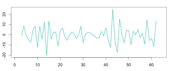
1 2 | random_air = timeserie_air / (trend_air * seasonal_air) plot(as.ts(random_air)) |
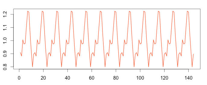
Step 6: Reconstruct the Original Signal
The decomposed time series can logically be recomposed using the model formula to reproduce the original signal. Some data points will be missing at the beginning and the end of the reconstructed time series, due to the moving average windows which must consume some data before producing average data points.
Additive
The additive formula is “Time series = Seasonal + Trend + Random”, which means “Random = Time series – Seasonal – Trend”
Multiplicative
The multiplicative formula is “Time series = Seasonal * Trend * Random”, which means “Random = Time series / (Trend * Seasonal)”
1 2 | recomposed_beer = trend_beer+seasonal_beer+random_beer plot(as.ts(recomposed_beer)) |
1 2 | recomposed_air = trend_air*seasonal_air*random_air plot(as.ts(recomposed_air)) |
DECOMPOSE( ) and STL(): Time Series Decomposition in R
To make life easier, some R packages provides decomposition with a single line of code. As expected, our step-by-step decomposition provides the same results as the DECOMPOSE( ) and STL( ) functions (see the graphs).
Additive
The only requirement: seasonality is quarterly (frequency = 4)
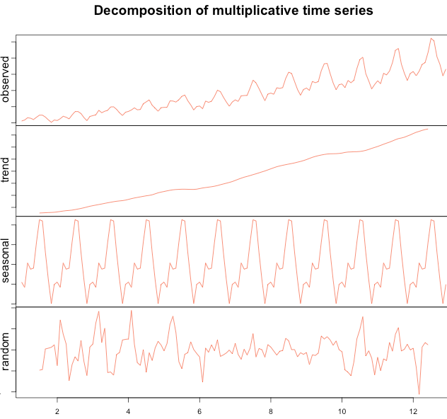
Using the DECOMPOSE( ) function:
Multiplicative
The only requirement: seasonality is monthly (frequency = 12)
1 2 3 4 5 6 7 | ts_beer = ts(timeserie_beer, frequency = 4) decompose_beer = decompose(ts_beer, "additive") plot(as.ts(decompose_beer$seasonal)) plot(as.ts(decompose_beer$trend)) plot(as.ts(decompose_beer$random)) plot(decompose_beer) |
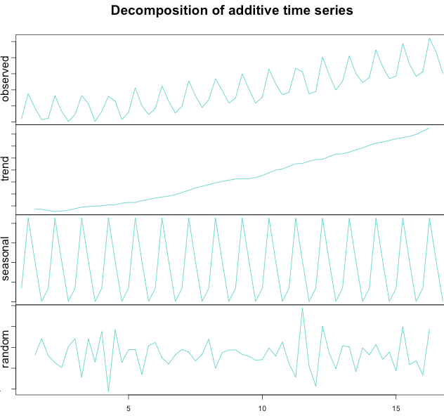
1 2 3 4 5 6 7 | ts_air = ts(timeserie_air, frequency = 12) decompose_air = decompose(ts_air, "multiplicative") plot(as.ts(decompose_air$seasonal)) plot(as.ts(decompose_air$trend)) plot(as.ts(decompose_air$random)) plot(decompose_air) |
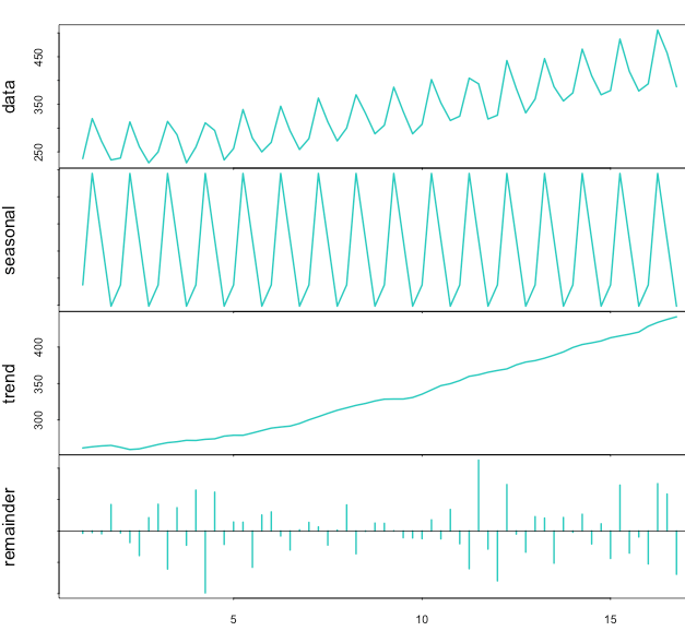
Now using the STL( ) function:
1 2 3 4 5 6 7 8 9 10 11 | ts_beer = ts(timeserie_beer, frequency = 4) stl_beer = stl(ts_beer, "periodic") seasonal_stl_beer <- stl_beer$time.series[,1] trend_stl_beer <- stl_beer$time.series[,2] random_stl_beer <- stl_beer$time.series[,3] plot(ts_beer) plot(as.ts(seasonal_stl_beer)) plot(trend_stl_beer) plot(random_stl_beer) plot(stl_beer) |
Conclusion
Decomposition is often used to remove the seasonal effect from a time series. It provides a cleaner way to understand trends. For instance, lower ice cream sales during winter don’t necessarily mean a company is performing poorly. To know whether or not this is the case, we need to remove the seasonality from the time series. Here, at Anomaly.io we detect anomalies, and we use seasonally adjusted time series to do so. We also use the random (also call remainder) time series from the decomposed time series to detect anomalies and outliers.
Monitor & detect anomalies with Anomaly.io
SIGN UP sending...