Time series decomposition splits a time series into seasonal, trend and random residual time series. The trend and the random time series can both be used to detect anomalies. But detecting anomalies in an already anomalous time series isn’t easy.
TL;DR
When working on an anomalous time series:
- Anomaly detection with moving average decomposition doesn’t work
- Anomaly detection with moving median decomposition works
The Problem with Moving Averages
In the blog entry on time series decomposition in R, we learned that the algorithm uses a moving average to extract the trends of time series. This is perfectly fine in time series without anomalies, but in the presence of outliers, the moving average is seriously affected, because the trend embeds the anomalies.
In this demonstration, we will first detect anomalies using decomposition with a moving average. We’ll see that this doesn’t work well, and so will try detecting anomalies using decomposition with a moving median to get better results.
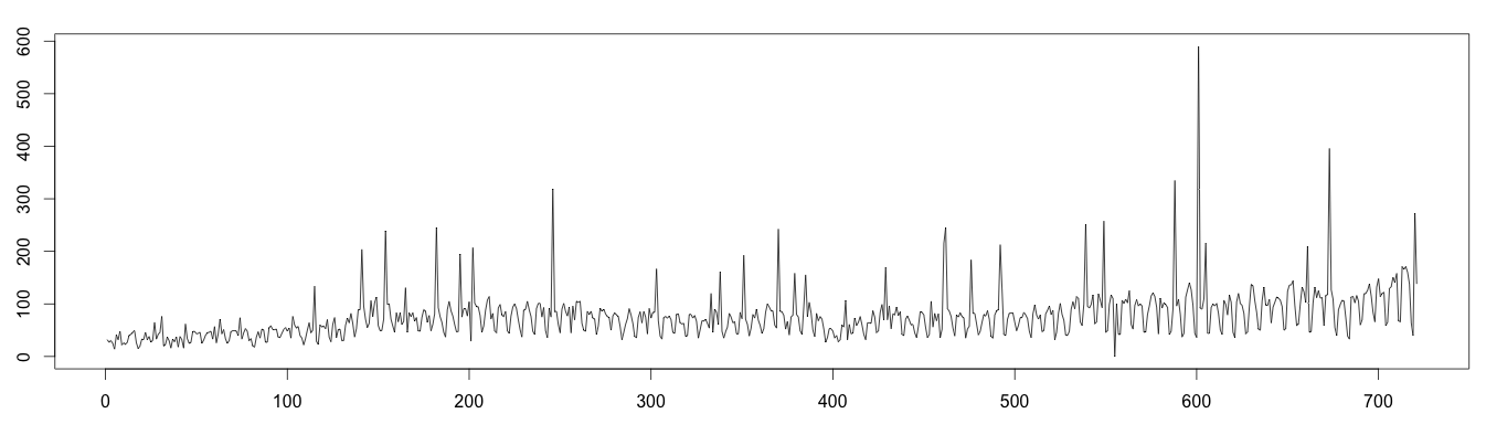
About the data: webTraffic.csv reports the number of page view per day over a period of 103 weeks (almost 2 years). To make the data more interesting, we added some (extra) anomalies to it. Looking at the time series, we clearly see a seasonality of 7 days; there is less traffic on weekends.
To decompose a seasonal time series, the seasonality time period is needed. In our example, we know the seasonality to be 7 days. If unknown, it is possible to determine the seasonality of a time series. Last but not least, we need to know if the time series is additive or multiplicative. Our web traffic is multiplicative.
To sum up our web traffic:
- Seasonality of 7 days (over 103 weeks)
- Multiplicative time series
- Download here: webTraffic.csv
1 2 3 4 5 6 7 8 9 | set.seed(4) data <- read.csv("webTraffic.csv", sep = ",", header = T) days = as.numeric(data$Visite) for (i in 1:45 ) { pos = floor(runif(1, 1, 50)) days[i*15+pos] = days[i*15+pos]^1.2 } days[510+pos] = 0 plot(as.ts(days)) |
Moving Average Decomposition (Bad Results)
Before going any further, make sure to import the data. Also, I recommend being sure that you understand how time series decomposition works. The stats package provides the handy decompose function in R.
1 – Decomposition
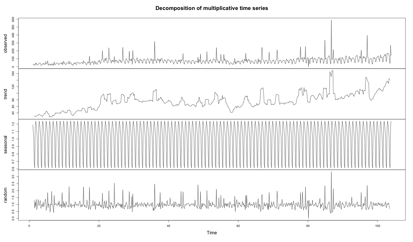
As the time series is anomalous during the decomposition, the trends become completely wrong. Indeed, the anomalies are averaged into the trend.
1 2 3 4 5 6 | # install required library install.packages("FBN") library(FBN) decomposed_days = decompose(ts(days, frequency = 7), "multiplicative") plot(decomposed_days) |
2 – Using Normal Distribution to Find Minimum and Maximum
To the random noise we can apply the normal distribution to detect anomalies. Values under or over 4 times the standard deviation can be considered outliers.
1 2 3 4 5 6 7 | random = decomposed_days$random min = mean(random, na.rm = T) - 4*sd(random, na.rm = T) max = mean(random, na.rm = T) + 4*sd(random, na.rm = T) plot(as.ts(as.vector(random)), ylim = c(-0.5,2.5)) abline(h=max, col="#e15f3f", lwd=2) abline(h=min, col="#e15f3f", lwd=2) |
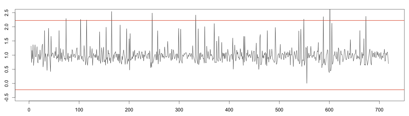
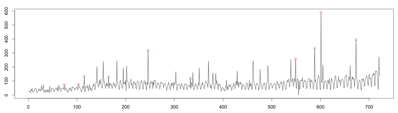
3 – Plotting Anomalies
Let’s find the values either over or under 4 standard deviations to plot the anomalies. As expected, the calculation fails to find many anomalies, due to the use of moving average by the decomposition algorithm.
1 2 3 4 5 6 7 8 9 10 11 12 13 14 | #find anomaly position = data.frame(id=seq(1, length(random)), value=random) anomalyH = position[position$value > max, ] anomalyH = anomalyH[!is.na(anomalyH$value), ] anomalyL = position[position$value < min, ] anomalyL = anomalyL[!is.na(anomalyL$value), ] anomaly = data.frame(id=c(anomalyH$id, anomalyL$id), value=c(anomalyH$value, anomalyL$value)) anomaly = anomaly[!is.na(anomaly$value), ] plot(as.ts(days)) real = data.frame(id=seq(1, length(days)), value=days) realAnomaly = real[anomaly$id, ] points(x = realAnomaly$id, y =realAnomaly$value, col="#e15f3f") |
Moving Average Decomposition (Good Results)
In our second approach, we will do the decomposition using a moving median instead of a moving average. This requires understanding how the moving median is robust to anomalies and how time series decomposition works. Also, again make sure to import the data. The moving median removes the anomalies without altering the time series too much.
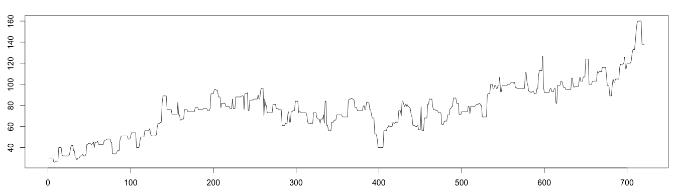
1 – Applying the Moving Median
The decomposed trend with moving median (see above graphic) is a bit “raw” but expresses the trend better.
1 2 3 4 5 6 7 | #install library install.packages("forecast") library(forecast) library(stats) trend = runmed(days, 7) plot(as.ts(trend)) |
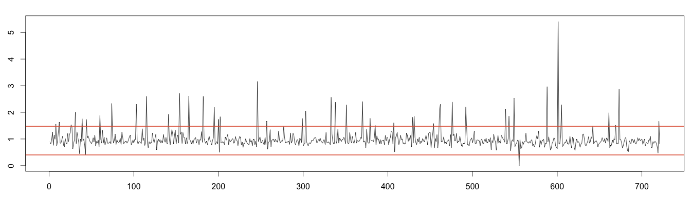
2 – Using the Normal Distribution to Find the Minimum and Maximum
As the decomposition formula expresses, removing the trend and seasonality from the original time series leaves random noise. As it should be normally distributed, we can apply the normal distribution to detect anomalies. As we saw previously, values under or over 4 times the standard deviation can be considered outliers. As random time series still contain the anomalies, we need to estimate the standard deviation without taking the anomalies into account. Once again, we will use the moving median to exclude the outliers.
1 2 3 4 5 6 7 8 9 10 11 | detrend = days / as.vector(trend) m = t(matrix(data = detrend, nrow = 7)) seasonal = colMeans(m, na.rm = T) random = days / (trend * seasonal) rm_random = runmed(random[!is.na(random)], 3) min = mean(rm_random, na.rm = T) - 4*sd(rm_random, na.rm = T) max = mean(rm_random, na.rm = T) + 4*sd(rm_random, na.rm = T) plot(as.ts(random)) abline(h=max, col="#e15f3f", lwd=2) abline(h=min, col="#e15f3f", lwd=2) |
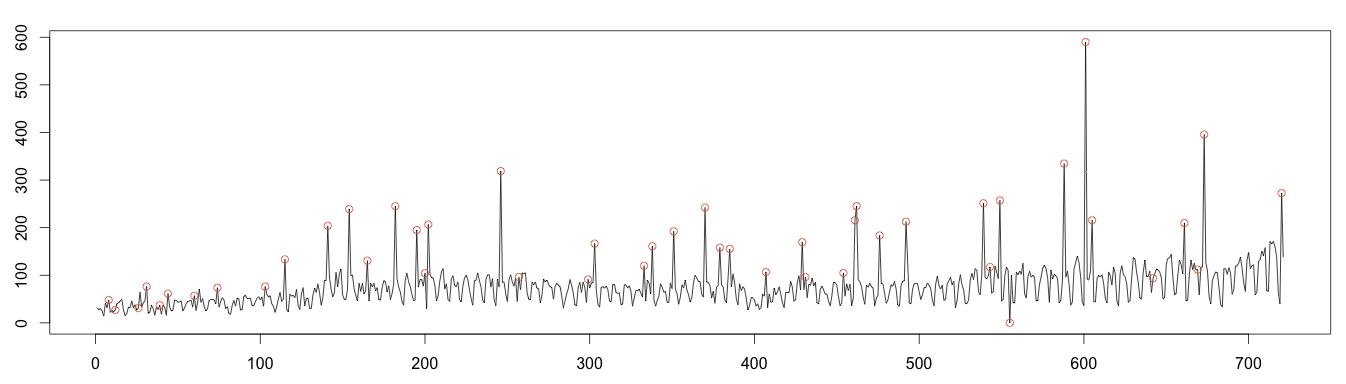
3 – Plotting Anomalies
As before, values over or under 4 times the standard deviation are plotted as anomalous. This works much better; we detect almost every anomaly! Once again, this is because the moving median is robust to anomalies.
1 2 3 4 5 6 7 8 9 10 11 12 13 14 | #find anomaly position = data.frame(id=seq(1, length(random)), value=random) anomalyH = position[position$value > max, ] anomalyH = anomalyH[!is.na(anomalyH$value), ] anomalyL = position[position$value < min, ] anomalyL = anomalyL[!is.na(anomalyL$value)] anomaly = data.frame(id=c(anomalyH$id, anomalyL$id), value=c(anomalyH$value, anomalyL$value)) points(x = anomaly$id, y =anomaly$value, col="#e15f3f") plot(as.ts(days)) real = data.frame(id=seq(1, length(days)), value=days) realAnomaly = real[anomaly$id, ] points(x = realAnomaly$id, y =realAnomaly$value, col="#e15f3f") |
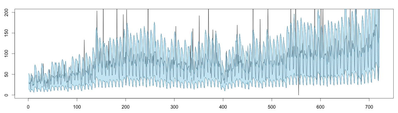
Here is an alternative plot displaying the same results: values outside the blue area can be considered anomalous.
1 2 3 4 5 6 7 8 9 10 11 | high = (trend * seasonal) * max low = (trend * seasonal) * min plot(as.ts(days), ylim = c(0,200)) lines(as.ts(high)) lines(as.ts(low)) x = c(seq(1, length(high)), seq(length(high), 1)) y = c(high, rev(low)) length(x) length(y) polygon(x,y, density = 50, col='skyblue') |
Monitor & detect anomalies with Anomaly.io
SIGN UP sending...