It is common to monitor the number of events that occur in a period of time. Unfortunately, this technique isn’t fast, and can fail to detect some anomalies. The alternative is to change the problem to studying the period of time between events.
Poisson Distribution Doesn’t Work
Traditional monitoring records the number of events for a period of time. There are two major problem with this approach:
- Due to randomness, it is difficult to spot an anomaly
- When the event rate is low, detection becomes very slow
Previously, we went into details and solved both problems by studying the period of time between events using the Poisson distribution to detect anomalies (please read this article, if you haven’t yet, before continuing). To apply the Poisson distribution we need to check if we are monitoring a Poisson process. For this to be the case, two conditions must hold.
1. Events need to occur independently
In server monitoring, events don’t always occur independently due to the underlying architecture. For example, when a user writes to a database table, other users can’t access the same table at the same time. They must wait in a queue. When the writer finishes, the queue is processed. This clearly shows a dependency of events so the Poisson distribution can’t be applied.
2. Average rate does not change
It is very common to see seasonal patterns in monitoring. Many servers are very busy during the day and much less at night. This change in rate doesn’t follow the Poisson process. A way to deal with this problem is to compare the average rate one week ago at the same time to predict today’s rate.
Using Percentile of Δt
Poisson anomaly detection was a perfect fit for analyzing time between events. Unfortunately, it doesn’t work in our case because our data aren’t Poisson distributed. Should we stop studying event rates and go back to event counts? Wait! Don’t give up yet, because there is a simple trick we can use. We are actually only interested in extremely rare event rates. So it doesn’t matter if this data isn’t Poisson distributed or normally distributed to detect anomalies. What really matters is to have a lower tail and/or upper tail with a very rare probability distribution.
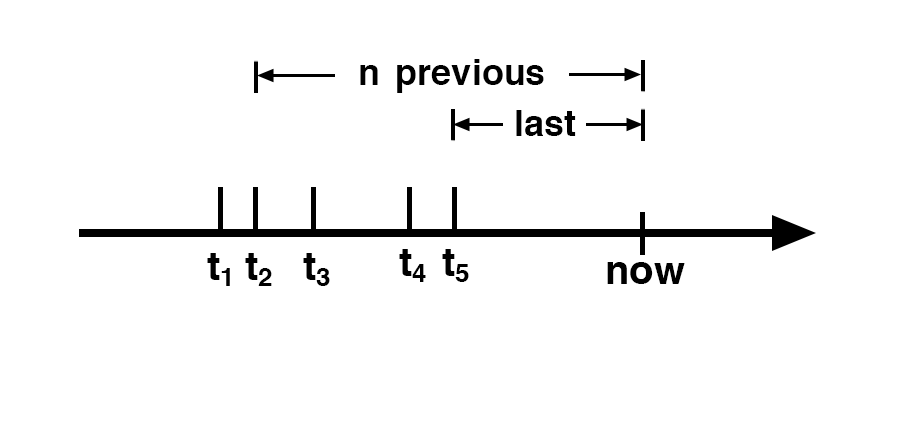
The main idea is to monitor the interval of time between the event at time t and the previous event at time t-1. The time difference between both events is known as Δt = t – t-1 .We can also monitor the time difference for the n previous events, which is Δt = t – t-n. Using n=1 will provide the fastest detection. Using n>1 allows detection of smaller rate variations, but requires some delay since it needs to wait for n events before anomaly detection.
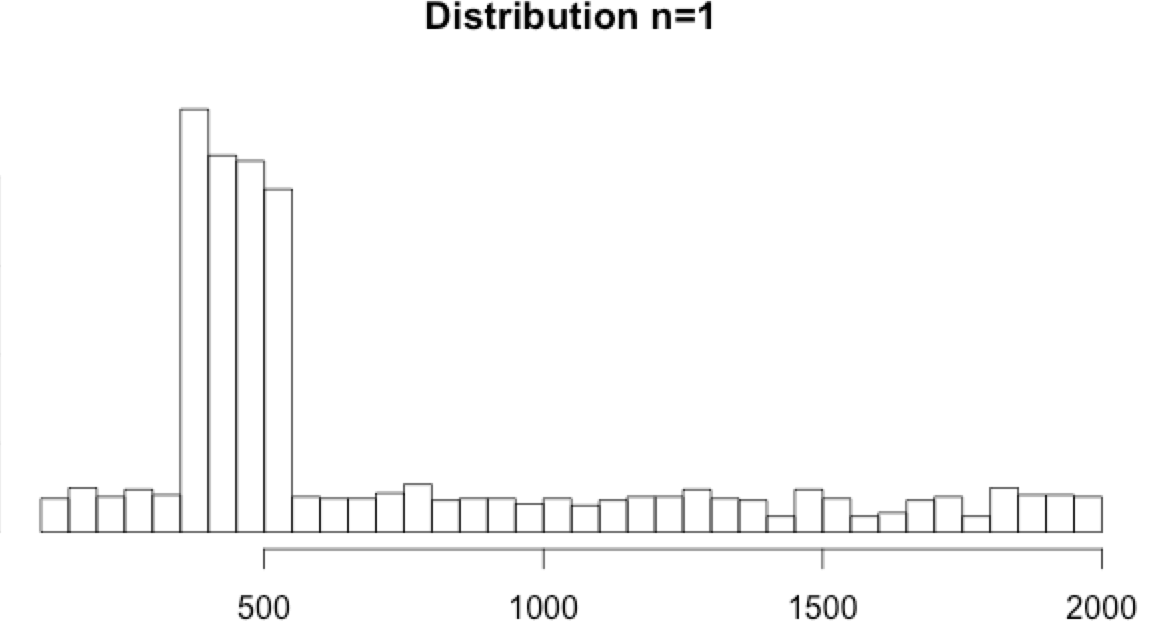
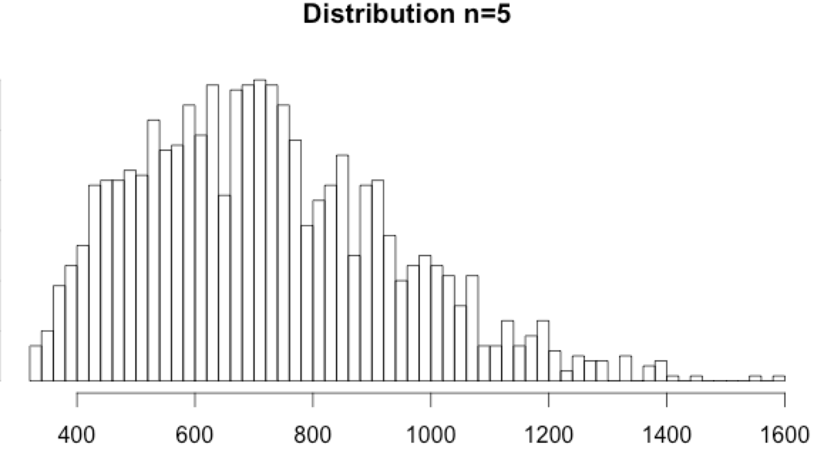
Download the data set recording event timestamps in milliseconds and the computed n=1, n=5 and n=10.
- The n=1 histogram doesn’t show any tail. Based on the distribution, the min and max values look impossible. But, as we don’t know the nature of the data, we will still apply min and max thresholds as a precaution.
- Interestingly, the n=5 and n=10 histograms do show a tail. It is neither Poisson distributed nor normally distributed, but extremely low or high values can be considered anomalies.
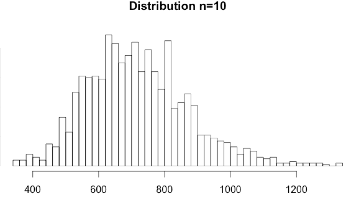
Using the 0.001 and 0.999 percentiles:
- for n=5, the percentiles are min=332 and max=1496
- for n=10, the percentiles are min=354 and max=1304
Please note that in this example data set the first 1500 events are normal before an anomaly append.
1 2 3 4 5 6 7 8 9 | v = read.csv('delta-record.csv', sep=';', stringsAsFactors=F); time = c(as.numeric(v[, 'time'])); n1 = c(as.numeric(v[, 'n1'])); n5 = c(as.numeric(v[, 'n5'])); n10 = c(as.numeric(v[, 'n10'])); qn1 = quantile(head(n1,1500), probs=c(0.001, 0.999), na.rm=T) qn5 = quantile(head(n5,1495), probs=c(0.001, 0.999), na.rm=T) qn10 = quantile(head(n10,1490), probs=c(0.001, 0.999), na.rm=T) |
Draw the data Δt and thresholds for different n:
1 2 3 4 5 6 7 8 9 10 | color = c("black", "#26c2b7", "#e05d38"); plot(x= tail(time, 150), y = tail(n1, 150), type = "l", ylim=c(0,2100), lwd=3, xlab = "time", ylab = "Δt"); lines(x= tail(time, 150), tail(n5, 150),col=color[2], lwd=3); lines(x= tail(time, 150), tail(n10, 150),col=color[3], lwd=3); abline(h=qn1, col=color[1], lwd=2); abline(h=qn5, col=color[2], lwd=2); abline(h=qn10, col=color[3], lwd=2); legend("topright", col=color, lwd=2, legend=c("n=1","n=5","n=10")); |
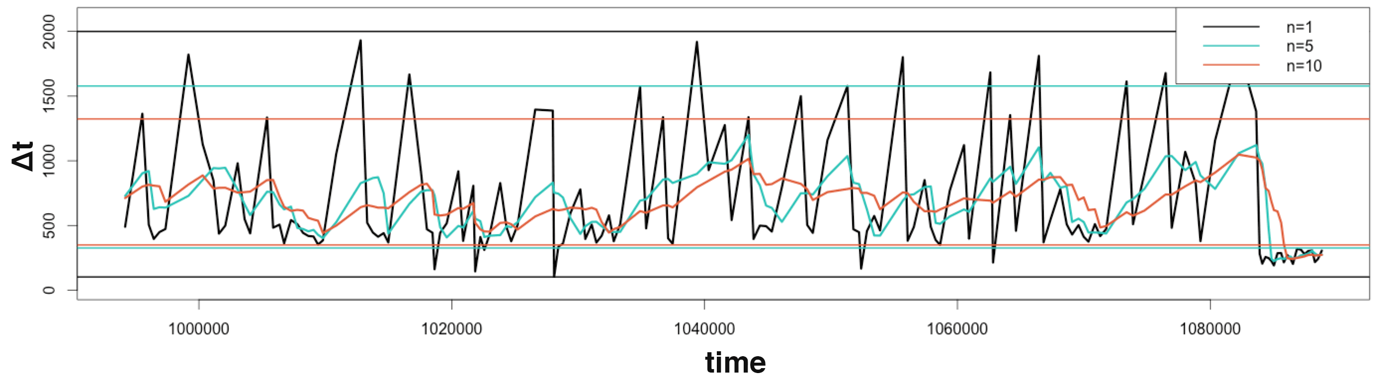 Note: Aggregated value was divided by n to appear on the same graph. The logic stay unchanged.
A small anomalous rate change occurs at the end of the graph:
- As discussed before, n=1 is very reactive, but it fails to detect the anomaly as every value are above its minimum limit.
- At the end of the graph, n=5 goes under its thresholds. It requires more delay than n=1 but at least it detected the anomalous change in the event rate.
- n=10 required even more time to detect the anomaly. It isn’t useful in this example, because it is far too slow. However, it could have been used to detect a change in rate that n=5 wouldn’t have found.
As already explained, n=1 provide the fastest detection, but fails to detect smaller unusual rate variations. The bigger n is, the more anomalies it will detect by smoothing the variations, unfortunately at the price of speed.
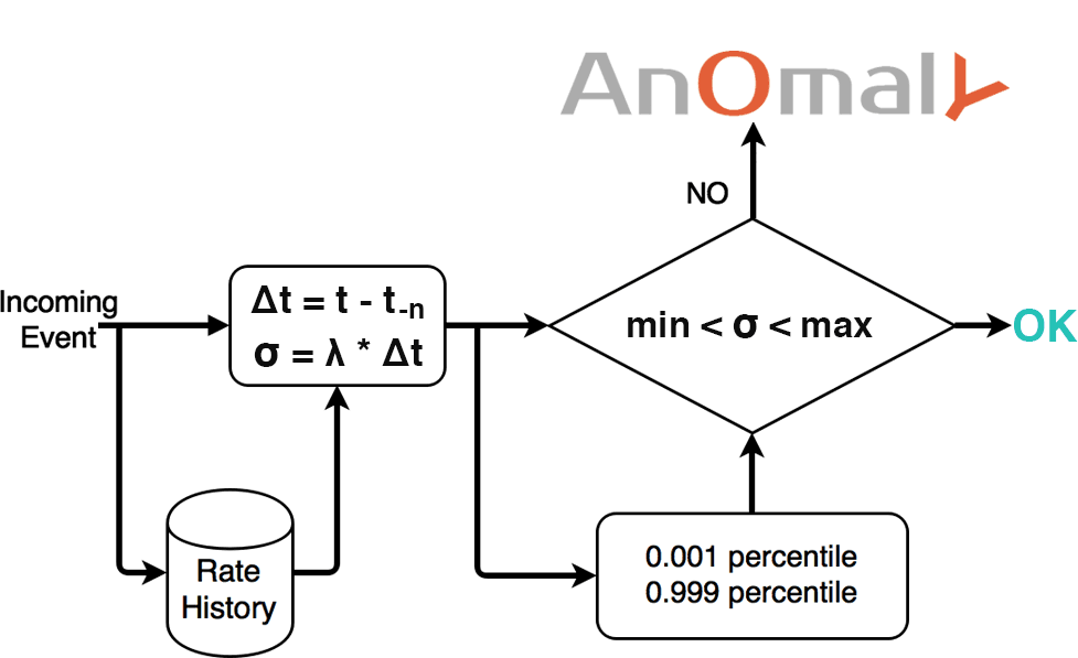
Including Event Rate λ
Usually, some change in rate will be noticed during monitoring. The event rate might even change a lot between day and night. Previously, we omitted such seasonality to calculate the thresholds, but as it happens, it is easy to integrate the event rate λ and to normalize the result. It is as simple as multiplying the event rate λ by the events’ time difference Δt. The result is σ = λ * Δt. The value σ is just a normalized version of Δt, so we can apply the percentile technique exactly how we did before.
The main difficulty is to have a correct estimate of λ. Based on the metric history, it might be possible to pick the previous rate exactly one week from now; this can work perfectly in some cases. In complex cases, picking λ might be hard, but that is beyond the scope of this article.
As explained in the chart, for each incoming event t :
- Select the event rate λ as it was one week ago
- Calculate the time difference Δt between event t and event t-n
- Multiply Δt and λ to find σ
- if σ is lower than the 0.001 percentile or higher than 0.999 percentile the event is an anomaly!
Implementation
Previously we learned how to make a Δt anomaly detection. Let’s now build a simple prototype in Java 8 using Joda time and CircularFifoQueue from Apache collections4. CircularFifoQueue is a “first in first out” queue that retains only the last x elements inserted: very useful for storing our n events.
As explained above, when an event occurs, we check if the rate stays between the min and max percentile. But how do we detect a total cessation, when no events occur at all? The trick is to check the queue every 10 ms by introducing a virtual event with the current date. This virtual event doesn’t get stored in the queue; it is only used to check every 10 ms if the rate goes too low. In the following implementation, this is the autoCheck.
The Detection class takes three arguments:
- List<Rule> min and max percentile of n
- RateHistory predicts the current rate λ
- autoCheck checks every 10 ms if the min rate is reached
The heart of the code is in the small detect function that calculates and checks σ from Δt and λ.
1 2 3 4 5 6 7 8 9 10 11 12 13 14 15 16 17 18 19 20 21 22 23 24 25 26 27 28 29 30 31 32 33 34 35 36 37 38 39 40 41 42 43 44 45 46 47 48 49 50 51 52 53 54 55 56 57 58 59 60 61 62 63 64 65 66 67 68 69 70 71 72 73 74 75 76 77 78 79 | //Detection.java import java.util.List; import java.util.Date; import java.util.Timer; import java.util.TimerTask; import org.apache.commons.collections4.queue.CircularFifoQueue; import org.joda.time.Interval; public class Detection { private CircularFifoQueue queue; private List rules; private RateHistory rateHistory; public Detection(List rules, RateHistory rateHistory, boolean autoCheck){ this.rules = rules; this.rateHistory = rateHistory; queue = new CircularFifoQueue(rules.get(rules.size()-1).n); if(autoCheck){ autoCheckEveryMillis(10); } } private void autoCheckEveryMillis(int millis) { Detection me = this; new Timer().schedule(new TimerTask() { public void run() { me.checkAllNoEvent(); } }, 0, millis); } public void newEvent(){ queue.add(new Date()); checkAllEvent(); } public void checkAllEvent(){ for(Rule rule : this.rules){ if(queue.size() >= rule.n){ checkEvent(rule); } } } public void checkAllNoEvent(){ for(Rule rule : this.rules){ if(queue.size() >= rule.n){ checkNoEvent(rule); } } } private void checkEvent(Rule rule){ Date last = queue.get(queue.size()-1); Date previous = queue.get(queue.size()-rule.n); detect(rule, last, previous); } public void checkNoEvent(Rule rule){ Date last = new Date(); Date previous = queue.get(queue.size()-rule.n+1); detect(rule, last, previous); } private void detect(Rule rule, Date last, Date previous){ float deltaT = delta(previous, last); float omega = this.rateHistory.predictCurrent() * deltaT; if(rule.minPercentile > omega){ System.out.println("ANOMALY - rate to low - found by n="+rule.n); }else if(omega > rule.maxPercentile){ System.out.println("ANOMALY - rate to high - found by n="+rule.n); } } private long delta(Date from, Date to){ Interval interval = new Interval(from.getTime(), to.getTime()); return interval.toDurationMillis(); } } |
1 2 3 4 5 6 7 8 9 10 11 12 13 14 15 16 17 18 19 20 21 22 23 24 25 26 27 28 29 30 31 32 33 34 35 36 37 38 39 40 41 42 43 44 45 46 47 48 49 50 51 52 53 54 55 56 57 58 59 | //Rule.java import java.util.Date; public class Rule { public Date date = new Date(); public int n; public float minPercentile; public float maxPercentile; public Rule(int n, float min, float max){ this.n = n; this.minPercentile = min; this.maxPercentile = max; } } //FakeRate.java public class FakeRate implements RateHistory { private boolean isNight = false; @Override public int predictCurrent() { if(isNight){ return 1; }else{ return 10; } } public void setInNightTime(){ isNight = true; } public void setInDayTime(){ isNight = false; } } //RateHistory.java public interface RateHistory { public int predictCurrent(); } //Rule.java import java.util.Date; public class Rule { public Date date = new Date(); public int n; public float minPercentile; public float maxPercentile; public Rule(int n, float min, float max){ this.n = n; this.minPercentile = min; this.maxPercentile = max; } } |
Let’s try this code with two already calculated n:
- n=5 with a min and max percentile 3650 and 4750
- n=10 with a min and max percentile 8100 and 9800
For this example, we created a FakeRate class. It will predict a rate of λ=10 events during daytime and λ=1 events during nighttime.
1 2 3 4 5 6 7 8 9 10 11 12 13 14 15 16 17 18 19 20 21 22 23 24 25 26 27 28 29 30 31 32 33 34 35 36 37 38 39 40 41 42 43 44 45 46 47 48 | //Main.java import java.util.ArrayList; import java.util.List; public class Main { private void sendEvent(Detection detection, int rate) throws InterruptedException { for(int i=0; i<10; i++){ Thread.sleep(rate); detection.newEvent(); } } public void run() throws InterruptedException { List rules = new ArrayList(); rules.add(new Rule(5, 3650, 4750)); rules.add(new Rule(10, 8100, 9800)); FakeRate rate = new FakeRate(); Detection detect = new Detection(rules, rate, false); System.out.println("NIGHT TIME"); rate.setInNightTime(); sendEvent(detect, 1000); System.out.println("* set anomaly too slow..."); sendEvent(detect, 850); System.out.println("* back to normal"); sendEvent(detect, 1000); System.out.println("* set anomaly too fast..."); sendEvent(detect, 1100); System.out.println("\n\rDAY TIME"); rate.setInDayTime(); System.out.println("* back to normal"); sendEvent(detect, 100); System.out.println("* set anomaly too fast..."); sendEvent(detect, 75); // Check rules break down System.out.println("\n\rWITH AUTOCHECK"); Detection detect2 = new Detection(rules, rate, true); sendEvent(detect2, 1000); System.out.println("* set anomaly break..."); Thread.sleep(110000); } public static void main(String[] args) throws Exception { new Main().run(); } } |
First anomaly:
- n=5 detects the anomaly quite fast
- n=10 requires 4 extra events to detect it
Second anomaly:
- The change in rate is too small for n=5 to detect
- n=10 detects the problem after 12 (small) anomalous events
When transiting to “daytime,” many anomalies are detected. This is because our rate becomes 10x faster. In reality, this should be a smoother transition, so it shouldn’t trigger any alert.
The third anomaly:
- n=5 detects the anomaly quickly
- n=10 requires 2 extra events to detect it
In the last part, we create an anomaly detection without sending any event. Since the autoCheck is enabled (as it always should be), it detects the low rate within 10 ms.
Conclusion
As discussed in detail when building an anomaly detection using the Poisson-distribution, focusing on the event rate will detect anomalies very quickly. Under high rates, a few milliseconds can be enough to spot an anomaly.
Anomaly detection studies outliers: It doesn’t matter what the distribution is as long as outliers are detected. When plotting the distribution, a tail or two might become visible. The upper tail can be used to detect a “too high” rate change, the lower tail a “too low” rate change. If no tail is present, choose higher values of n. Still no tail in sight? Maybe you should consider other anomaly detection techniques…
The key to success of this anomaly detection technique is to very carefully choose the rate predictor λ. As every calculation depends on the λ prediction, picking the wrong value will result in many false positives.
Monitor & detect anomalies with Anomaly.io
SIGN UP sending...